Statistics & Regression
State all assumptions, show all calculations.
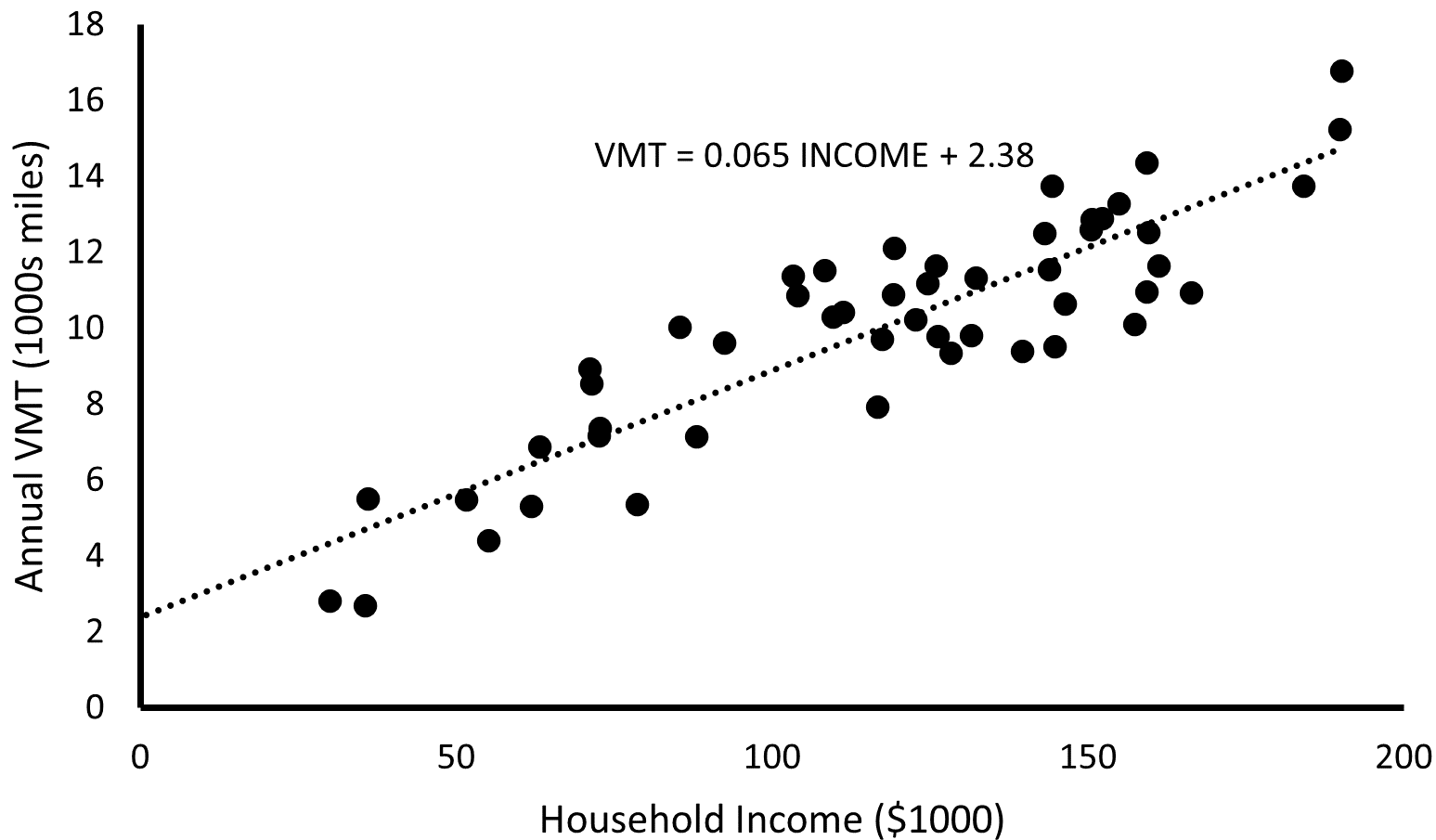
- The below figure shows data corresponding to the fitted line y = 0.065x + 2.38 with residual standard deviation 1.42. The residual standard deviation is a measure of remaining variation not captured by the regression model. The range of income is roughly between $29,000 and $195,000.
- Sketch hypothetical data (in pen or pencil) with the same range of x (income) but corresponding to the line y = 0.065x + 1.25 with residual standard deviation 1.42.
- Sketch hypothetical data (in a different color than in part a) with the same range of x (income) but corresponding to the line y = 0.065x + 1.25 with residual standard deviation 5.0. Note: negative VMT values are fine for this exercise.
- Give examples of applied statistics problems of interest to you in which the goals are:
- Forecasting/classification
- Exploring associations
- Extrapolation
- Causal inference
- A survey is conducted in a certain state regarding support for increasing the gas tax to fund transportation investments. In this survey, a higher tax is supported by 50% of respondents aged 18-29, 60% of respondents aged 30-44, 25% of respondents aged 45-64, and 10% of respondents aged 65 and up. Use the weighted average formula (available in many places online) to compute the proportion of respondents in the sample who support a higher tax. Assume there is no nonresponse.
- For the sample: Suppose the sample includes 50 respondents aged 18-29, 300 aged 30-44, 275 aged 45-64, and 375 aged 65+.
- For the Nebraska population: Assume the state where the survey was performed is Nebraska. How would you adjust your weighted average to represent the population? Assume the following population distribution for the state.
| Age group | NE population |
|---|---|
| 18-29 | 265260 |
| 30-44 | 368768 |
| 45-64 | 458101 |
| 65+ | 312458 |
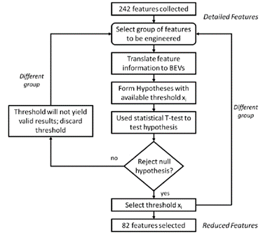
- An analyst is interested in the relationship between demographic features and electric vehicle (EV) adoption. They develop a procedure to determine variables that might affect adoption (see figure below). Their procedure starts with 242 features (variables), which they narrow to 82 features using t-test statistics. In the below figure, the term “features to be engineered” simply refers to combining and transforming variables to reduce the number of features and/or their correlation. As a hint, this study was chosen as an example of low-quality analysis. There may be no clear interpretation to a figure, and it is acceptable to state this conclusion.
- Please comment on the validity of this procedure. Note: There is no single solution to this problem. The goal is to start thinking about data analysis.
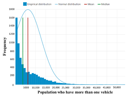
- The analyst generates the following figure. What information is provided by this figure? Is its implication evident from the available information? What additional information would help to clarify its interpretation?